本文主要是简单的构建了一个分类器。首先是针对iris数据集,构建了一个只用阈值来分类的情况。之后简介了下交叉验证。然后考虑了更实际的数据集,使用了UCI的数据集,并考虑特征处理,使用logistics回归分类。最后,简单的说了一下分析的思路和一些待思考的问题。这里数据集和问题是参考了书籍《building machine learning system with python》,建模过程和分析属于个人见解,请批判阅读。
目录
1、简单分类器
首先我们导入一些我们需要使用的库。这里主要是使用python,以及它的一些包,主要是numpy、scipy、sklearn等等,绘图使用matplotlib,这里我个人习惯采用ggplot的配色风格。在最开始,我们新可视化一下数据,做一些基本的数据探索。
import numpy as np
from sklearn.datasets import load_iris
from matplotlib import pyplot as plt
import pandas as pd
%matplotlib inline
import seaborn as sns
# styles = ["white", "dark", "whitegrid", "darkgrid", "ticks"]
sns.set(style="darkgrid")

iris = sns.load_dataset("iris")
sns.pairplot(iris, hue="species", size=3.0)
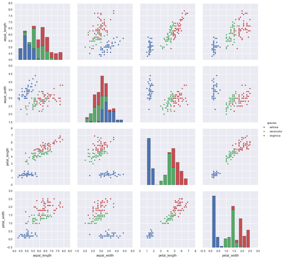
如果我们只有选择一个特征作为分类特征,选择一个阈值,我们以最后一幅图为例,可以选择petal的长度,取4.8为阈值(可以设定不同的阈值,看看那个阈值分类最高,图里可以看到绿色的最大值作为分割点是最优的)。这个没啥意思,不过也提供了一种简单的分析思路。我主要想做这个图看看而已。
2、logistic回归
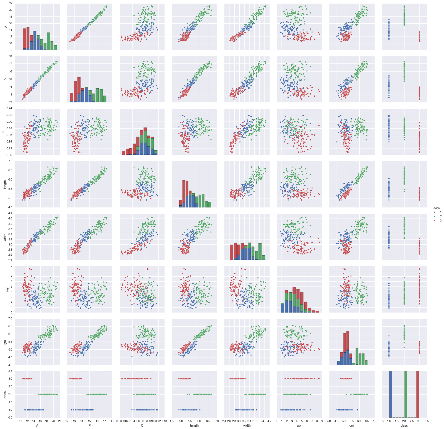
这里使用了新的数据集,是小麦种子数据。有7个特征,area A(面积), perimeter P(周长), compactness C = 4piA/P\^2(紧密度), length of kernel(胚长度), width of kernel(胚宽度), asymmetry coefficient(偏度系数), length of kernel groove(胚槽长度)。
seeds = pd.read_excel('seeds_dataset.xlsx', names=['A','P','C','length','width','asy', 'gro','class'], header=None)
seeds.describe()
| A | P | C | length | width | asy | gro | class | |
|---|---|---|---|---|---|---|---|---|
| count | 210 | 210 | 210 | 210 | 210 | 210 | 210 | 210 |
| mean | 14.84 | 14.55 | 0.87 | 5.62 | 3.25 | 3.70 | 5.40 | 2.00 |
| std | 2.90 | 1.30 | 0.02 | 0.44 | 0.37 | 1.50 | 0.49 | 0.81 |
| min | 10.59 | 12.41 | 0.80 | 4.89 | 2.63 | 0.76 | 4.51 | 1.00 |
| 25% | 12.27 | 13.45 | 0.85 | 5.26 | 2.94 | 2.56 | 5.04 | 1.00 |
| 50% | 14.35 | 14.32 | 0.87 | 5.52 | 3.23 | 3.59 | 5.22 | 2.00 |
| 75% | 17.30 | 15.71 | 0.88 | 5.97 | 3.56 | 4.76 | 5.87 | 3.00 |
| max | 21.18 | 17.25 | 0.91 | 6.67 | 4.03 | 8.45 | 6.55 | 3.00 |
sns.pairplot(seeds, hue="class", size=2.5)
f, ax = plt.subplots(figsize=(7, 7))
cmap = sns.diverging_palette(220, 10, as_cmap=True)
sns.corrplot(seeds, annot=True, sig_stars=False,
             diag_names=False, cmap=cmap, ax=ax)
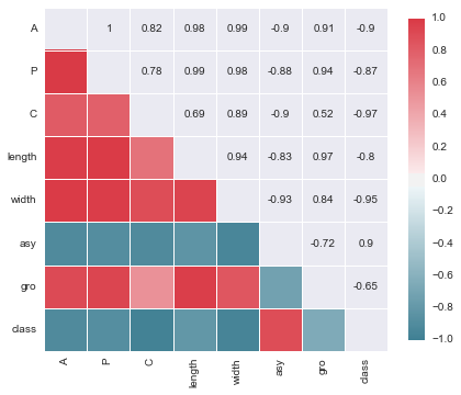
原始数据中,部分分隔符错乱,所以我们转成了excel。通过数据描述,我们发现都是数值的,且没有缺失值,但单位不一。另外,各个变量之间的相关关系很明显。 所以,我们考虑先使用一些模型来做分类,使用交叉验证,看看结果如何。如果效果不好,使用归一化以及做一些特征选择,再看看效果。 此外,这里我们使用两类模型,一类是可解释的,一类是注重分类精度的。
from sklearn import cross_validation as c_v
from sklearn import svm
from sklearn import linear_model

# svm model
# we can choose some feature for the model, based on the corrplot, we could drop the "P"
# and in this part, we use all the features.
feature = ['A','P','C','length','width','asy', 'gro'] # ['A','P','C','length','width','asy', 'gro']
for i in range(1, 11):
    i = float(i) / 10
    model_svm = svm.SVC(C=i)
    score_svm = c_v.cross_val_score(model_svm, seeds[feature], seeds['class'], cv=10)
    print 'svm: with the C={c}, the score is {s:.3}, var is {v:.3}'.format(c=i, s=score_svm.mean(), v=score_svm.var())

model_lr = linear_model.LogisticRegression()
score_lr = c_v.cross_val_score(model_lr, seeds[feature], seeds['class'], cv=10)
print 'LogisticRegression: the score is {s:.3}, var is {v:.3}'.format(s=score_lr.mean(), v=score_lr.var())
我们看到使用了SVM等方法,发现使用LogisticRegression的结果可以达到92.4%,而且方差也比较小。那么,接下来我们只用LogisticRegression进行分析,毕竟LogisticRegression的可解释比较强。我们做一些特征变换和特征选择。这里,我们先采用归一化。这里为了方便,我们直接把数据集分割为训练数据和测试数据。
3、归一化与增加特征
from sklearn import preprocessing as pps
X_train, X_test, y_train, y_test = c_v.train_test_split(seeds.iloc[:,:-1], seeds['class'], test_size=0.2, random_state=1234)
scaler = pps.StandardScaler().fit(X_train) #StandardScaler(), MinMaxScaler() , Normalizer()

model_lr1 = linear_model.LogisticRegression()
model_lr1.fit(X_train, y_train)
print model_lr1.score(X_train, y_train), model_lr1.score(X_test, y_test)

model_lr2 = linear_model.LogisticRegression()
model_lr2.fit(scaler.transform(X_train), y_train)
print model_lr2.score(scaler.transform(X_train), y_train), model_lr2.score(scaler.transform(X_test), y_test)

# just for a test
model_lr = linear_model.LogisticRegression()
scaler = pps.StandardScaler().fit(seeds.iloc[:,:-1])
score_lr1 = c_v.cross_val_score(model_lr, seeds.iloc[:,:-1], seeds['class'], cv=10)
score_lr2 = c_v.cross_val_score(model_lr, scaler.transform(seeds.iloc[:,:-1]), seeds['class'], cv=10)

print 'the score is {s:.3f}, var is {v:.5f}'.format(s=score_lr1.mean(), v=score_lr1.var())
print 'the score is {s:.3f}, var is {v:.5f}'.format(s=score_lr2.mean(), v=score_lr2.var())

print 'weight for class0:{0[0]:.3}, {0[1]:.3}, {0[2]:.3}, {0[3]:.3}, {0[4]:.3}, {0[5]:.3}, {0[6]:.3}'.format(model_lr2.coef_[0])
print 'weight for class1:{0[0]:.3}, {0[1]:.3}, {0[2]:.3}, {0[3]:.3}, {0[4]:.3}, {0[5]:.3}, {0[6]:.3}'.format(model_lr2.coef_[1])
print 'weight for class2:{0[0]:.3}, {0[1]:.3}, {0[2]:.3}, {0[3]:.3}, {0[4]:.3}, {0[5]:.3}, {0[6]:.3}'.format(model_lr2.coef_[2])
print model_lr2.coef_.sum(axis=0), model_lr2.coef_.var(axis=0)
在分割之后,我们对比归一化和不归一化的结果,大约提升了进2.4个百分点。当然啦,这里啰嗦了一下,把直接使用所有数据进行交叉验证的结果放了进来(这样好像更有说服力,但是,这里的归一化确是有一点问题的)。这里是因为数据集比较小,所以多做了一些测试。如果是数据集比较大的话,再使用交叉验证就非常费时间,一般直接把数据集随机分割,也能说明问题。
此外,我们输出了对应类别下的权重值。这里提到在上一步特征选择,从corrplot可以看出,变量之间是存在相关性的。但是,这些相关是在无视类别的情况的。如果在同一类别中,变量之间的相关性就会发生变化,这里使用命令pd.DataFrame(X_train[y_train==1]).corr()就可以看到,一些变量之间的关系不再赘述。
那么我们想再提高几个百分点怎么办?这里简单的分析一下,通过分析发现,测试误差(泛化误差)小于训练误差,可以认为没有过拟合。而训练准确度达到了90%以上,那么模型的偏差(bias)也比较小,想再降低偏差,可以增加一些特征,或者增加样本等等方法。这里我们选择适当的考虑增加一些变量,比如第二列是周长P,那么我们增加这一列的开方,情况会怎么样呢?或者增加一些平方项呢?这种特征变换,通常会有一些有趣的结果,比如增加紧密度和胚槽长度)的平方、开方项,对结果的提升较好。这里不再一一举例,各位可以去尝试,比如删除一些列,或者增加一些特征乘积项等等。下面的脚本里,把这种增加的方法都写了出来,方便尝试和探索。最终,我们仍然要考虑特征的数量,可解释行等等。
这里,最后我们可以得到在不进行归一化后,只进行特征变换和增删,可以达到97.62%准确率(即使我们使用交叉验证,也可以达到97.1%,相比之前的90%有了很大的提升);而使用归一化后可以达到95.24%,这可能跟引入新的特征,变换幅度有问题,大家可以尝试部分特征的归一化。
# k is the colum we wanna add with the sqrt transform
# j is the colum we wanna add with the square transform
# r is the colum we wanna delete
k = [1,3,6] # k =[3, 6]
j = [3,6]
r = [2,3,6]
q = [[1,6]]
# area A(面积0), perimeter P(周长1), compactness C = 4piA/P^2(紧密度2), length of kernel(胚长度3),
# width of kernel(胚宽度4), asymmetry coefficient(偏度系数5), length of kernel groove(胚槽长度6)

X_train1 = X_train.copy()
tmp1 = np.sqrt(X_train[:,k]).reshape((X_train1.shape[0],len(k)))
tmp2 = np.square(X_train[:,j]).reshape((X_train1.shape[0],len(j)))
X_train1 = np.concatenate((X_train1, tmp1, tmp2), axis=1)
for i in q:
    tmp3 = np.multiply(X_train[:,i[0]], X_train[:,i[0]]).reshape((X_train1.shape[0],1))
    X_train1 = np.concatenate((X_train1, tmp3), axis=1)

X_train1 = np.delete(X_train1, r, axis=1)

X_test1 = X_test.copy()
tmp1 = np.sqrt(X_test[:,k]).reshape((X_test1.shape[0],len(k)))
tmp2 = np.square(X_test[:,j]).reshape((X_test1.shape[0],len(j)))
X_test1 = np.concatenate((X_test1, tmp1, tmp2), axis=1)
for i in q:
    tmp3 = np.multiply(X_test[:,i[0]], X_test[:,i[0]]).reshape((X_test.shape[0],1))
    X_test1 = np.concatenate((X_test1, tmp3), axis=1)

X_test1 = np.delete(X_test1, r, axis=1)

print X_train1.shape,X_test1.shape

scaler = pps.StandardScaler().fit(X_train1) #StandardScaler(), MinMaxScaler() , Normalizer()

model_lr1 = linear_model.LogisticRegression()
model_lr1.fit(X_train1, y_train)
print model_lr1.score(X_train1, y_train), model_lr1.score(X_test1, y_test)

model_lr2 = linear_model.LogisticRegression()
model_lr2.fit(scaler.transform(X_train1), y_train)
print model_lr2.score(scaler.transform(X_train1), y_train), model_lr2.score(scaler.transform(X_test1), y_test)

# just for a test
X =  seeds.iloc[:,:-1]
tmp1 = np.sqrt(X.iloc[:,k])
tmp2 = np.square(X.iloc[:,j])
X = np.concatenate((X, tmp1, tmp2), axis=1)
for i in q:
    tmp3 = np.multiply(X[:,i[0]], X[:,i[0]]).reshape((X.shape[0],1))
    X = np.concatenate((X, tmp3), axis=1)
X = np.delete(X, r, axis=1)
print X.shape

model_lr = linear_model.LogisticRegression()
scaler = pps.StandardScaler().fit(X)
score_lr1 = c_v.cross_val_score(model_lr, X, seeds['class'], cv=10)
score_lr2 = c_v.cross_val_score(model_lr, scaler.transform(X), seeds['class'], cv=10)
print 'the score is {s:.3f}, var is {v:.5f}'.format(s=score_lr1.mean(), v=score_lr1.var())
print 'the score is {s:.3f}, var is {v:.5f}'.format(s=score_lr2.mean(), v=score_lr2.var())
当然,我们也可以尝试Ensemble的方式。但是,这里只所以没有采用ensemble或者svm等方法,主要是为了可解释性。另外,使用Ensemble的话,通常可以得到一个更好的结果,但是在数据集比较大的时候,训练模型和调用模型的速度都会降低。当然,这是需要权衡的。有些问题方面,比如人脸检测,使用一些ensemble的框架,会比其他的方法有明显的提升。如果感兴趣的话,可以试一试使用ensemble的方法,看看是否有明显的提升呢?
那么,我们不禁要问为什么这样处理(增加平方项特征)是有效果的呢?增加特征,使得参数增加,模型的表达能力会有所增强,但是,不是说任意增减特征都会使得模型的表达能力增加。比如增加相同的一列,模型并不会提升明显(在交叉验证中,并没有提升,但是在某些场合,因为变量之间的相关性,得到结果有所变化),因为这里的权重信息并没有增加,模型的表达能力也不会有提升。
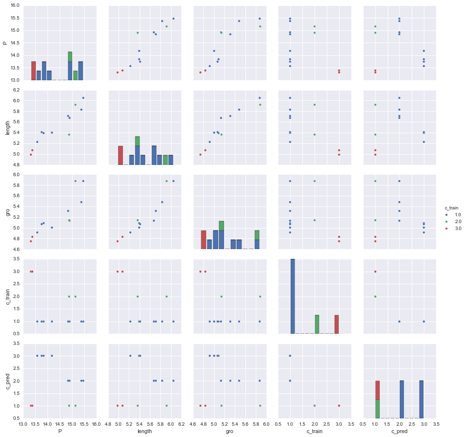
另外一个问题,为什么增加平方项或者增加一些乘积项呢?我们可以看一下错误分类的特征分布,进行分析。这里我们只用未经变换处理的数据。我们可以通过混淆矩阵(这里没给代码,直接把所有分类错误数据的feature输出了),可以看到分类错误的情况:多数是把原来为1的类别错误的分为了2和3。我们这里简单的分析一下,从最后一行,c_pred的和c_train下的各个特征,可以看到原来属于1类的,都被预测截断为2类和3,从图中看到,这要是因为这些1类的值范围比较大,覆盖了部分其他类(多数为2类)的值。对于某些2类值比较大的情况,我们可以考虑增加平方项,以此来拉开类别间的间距,这一点我们从权重值中也可以看出一点端倪,它对应的权重值比较大,方差也比较大,可以认为对分类比较重要,增加这种属性的特征变化,一般都会有好处。对于被截断的情况,我们可以考虑增加开方项,缩短截断长度。但是,这里隐含一个问题,就是我们这样的特征变换对原始正确分类的影响,因此也需要对比着最开始的pariplot进行思考,之后进行一定的尝试。当然,我个人在这方面也没有多少实际理论,这里都是个人理解而已,不能保证正确,大家自己琢磨。也不要为了得到一个可解释的结果,而强行去解释!
model_lr = linear_model.LogisticRegression()
model_lr.fit(X_train, y_train)
print model_lr.score(X_train, y_train), model_lr.score(X_test, y_test)
print 'weight for class0:{0[0]:.3}, {0[1]:.3}, {0[2]:.3}, {0[3]:.3}, {0[4]:.3}, {0[5]:.3}, {0[6]:.3}'.format(model_lr.coef_[0])
print 'weight for class1:{0[0]:.3}, {0[1]:.3}, {0[2]:.3}, {0[3]:.3}, {0[4]:.3}, {0[5]:.3}, {0[6]:.3}'.format(model_lr.coef_[1])
print 'weight for class2:{0[0]:.3}, {0[1]:.3}, {0[2]:.3}, {0[3]:.3}, {0[4]:.3}, {0[5]:.3}, {0[6]:.3}'.format(model_lr.coef_[2])
print model_lr.coef_.sum(axis=0), model_lr.coef_.var(axis=0)

y_pred = model_lr.predict(X_train)
error_choose = y_pred != y_train
error = X_train[error_choose,:]
c_pred = y_pred[error_choose].reshape(error.shape[0],1)
c_train = y_train[error_choose].reshape(error.shape[0],1)
error = np.concatenate((error,c_pred, c_train),axis=1)
f = [1,3,6,-1,-2]
name = ['A','P','C','length','width','asy', 'gro','c_pred','c_train']
error = pd.DataFrame(error[:,f],columns=[name[i] for i in f])
sns.pairplot(error, hue="c_train", size=2.5)
4、总结
最后,我们看一下整体。首先我们并没有完整的按照数据挖掘流程进行分析。这里,主要集中在建模的讨论中,而且毕竟是练习,所以也比较粗糙。简单的可视化了数据的情况,之后直接套模型看看效果,然后根据一些情况进行调整归一化和特征调整。有很多细节,我们可以深入的思考,比如得到的回归系数,我们如何解释?如果根据这些东西,进行调参呢?最后增加的特征,也只是简单的增加点,没有深入的探讨,当然也参考了数据的分布(pairplot图)。另外,在编程过程中,也需要注意内存的释放,这里因为数据集比较小,我没有使用delete variable来释放内存。还有有很多东西值得进一步的思考的东西,不再赘述!